(tl;dr: It's letter of recommendation season, and so I decided to write one to a paper that's really been influential in my recent thinking. Psychometrics, y'all.)
To whom it may concern:
I am writing to provide my strongest recommendation for the paper, "Attack of the Psychometricians" by Denny Borsboom (2006). Reading this paper oriented me to a rich tradition of psychometric modeling – but more than that, it changed my perspective on the relationship between psychological measurement and theory. (It also taught me to use the term "sumscore"* as an insult). I urge you to consider it for a position in your reading list, syllabus, or lab meeting.
I first met AotP (or Attack!, as I like to call it) via a link on twitter. Not the most auspicious beginning, but from a quick skim on my phone, I could tell that this was a paper that needed further study.
The paper presents and discusses what it calls the central insight of psychometrics: that "measurement does not consist of finding the right observed score to substitute for a theoretical attribute, but of devising a model structure to relate an observable to a theoretical attribute." In other words, the goal is to make models that link data to theoretical quantities of interest. What this means is that measurement is essentially continuous with theory construction. By creating and testing a good measurement model, you're creating and testing a key component of a good theory.
Tuesday, November 5, 2019
Tuesday, October 8, 2019
Confounds and covariates
(tl;dr: explanation of confounding and covariate adjustment)
Every year, one of the trickiest concepts for me to teach in my experimental methods course is the difference between experimental confounds and covariates. Although this distinction seems simple, it's pretty deeply related to the definition of what an experiment is and why experiments lead to good causal inferences. It's also caught up in a number of methodological problems that come up again and again in my class. This post is my attempt to explain the distinction and how it relates to different problems and cultural practices in psychology.
Throughout this post, I'll use a silly example. My first year of graduate school, I got distracted from my actual research by the hypothesis that listening to music with lyrics decreased my ability to write papers for my classes. I'll call this the "Bob Dylan" hypothesis, since I was listening to a lot of Dylan at the time. Let's represent this by the following causal diagram.

Our outcome is writing skill (Y) and our predictor is Dylan listening (X). The edge between them represents a hypothesized causal relationship. Dylan is hypothesized to affect writing skill, and not vice versa. (These kinds of diagrams are called causal graphical models*).
Observational Studies and Experiments
Suppose we did an observational study where we measured each of these variables in a large population. Assume we came up with some way to sample people's writing, get a measure of whether they either were or weren't listening to lyric-heavy music at the time, and assess the writing sample's quality. We might find that Y was correlated with X, but in a surprising direction: listening to Dylan would be related to better writing.
Can we make a causal inference in this case? If so, we could get rich promoting a Dylan-based writing intervention. Unfortunately, we can't – correlation doesn't equal causation here, because there is (at least one) confounding third variable: age (Z). Age is positively related to both Dylan listening and writing skill in our population of interest. Older people tend to be good writers and also tend to be more into folk rockers; I'm not even going to put a question mark on this edge because I'm pretty sure this is true.

But: the causal relationship of age to our other two variables means that variation in Z can induce a correlation in X and Y, even in the absence of a true causal link. We can say that age is a confound in estimating the Dylan-writing skill relationship: it's a variable that is correlated with both our predictor and our outcome variables.
To get gold-standard evidence about causality, we need to do an experiment. (We won't discuss statistical techniques for inferring causality, which can be useful but don't give you gold standard evidence anyway; review here).
Experiments are when we intervene on the world and measure the consequences. Here, this means forcing some people to listen to Dylan. In the language of graphical models, if we control the Dylan listening, that means that variable X is causally exogenous. (Exogenous means that it's not caused by anything else in the system). We "snipped" the causal link between age and Dylan listening.

So now we can "wiggle" the Dylan listening variable – change it experimentally – and see if we detect any changes in writing skill. We do this by randomly assigning individuals to listen to Dylan or not and then measuring writing during the assigned listening (or non-listening) period. This is a "between-subjects" design. We can use our randomized experiment to get a measure of the average treatment effect of Dylan, the size of the causal effect of the intervention on the outcome. In this simple experiment, the ATE is estimated by the regression Y ~ X (for ease of exposition, I'm not going to discuss so-called mixed models, which model variation across subjects and/or experimental items). That's the elegant logic of randomized experiments: the difference between condition gives you the average effect.
Confounds
Let's consider an alternate experiment now. Suppose we did the same basic procedure, but now with a "within-subjects" design where participants do both the Dylan treatment and the control, in that order. This experiment is flawed, of course. If you observe a Dylan effect, you can't rule out the idea that participants got tired and wrote worse in the control condition because it always came second.
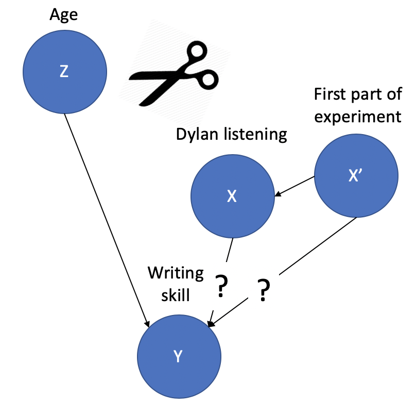
Order (Dylan first vs. control first; notated X') is an experimental confound: a variable that is created in the course of the experiment that is both causally related to the predictor and potentially also related to the outcome. Here's how the causal model now looks:

We've reconstructed the same kind of confounding relationship we had with age, where we had a variable (X') that was correlated both with our predictor (X) and our outcome (Y)! So...
What should we do with our experimental confounds?
Option 1. Randomize. Increasingly, this is my go-to method for dealing with any confound. Is the correct answer on my survey confounded with response side? Randomize what side the response shows up on! Is order confounded with condition? Randomize the order you present in! Randomization is much easier now that we program many of our experiments using software like Qualtrics or code them from scratch in JavaScript.
The only time you really get in trouble with randomization is when you have a large number of options, a small number of participants, or some combination of the two. In this case, you can end up with unbalanced levels of the randomized factors (for example, ten answers on the right side and two on the left). Averaging across many experiments, this lack of balance will come out in the wash. But in a single experiment, it can really mess up your data – especially if your participants notice and start choosing one side more than the other because it's right more often. For that reason, when balance is critical, you want option 2.
Option 2. Counterbalance. If you think a particular confound might have a significant effect on your measure, balancing it across participants and across trials is a very safe choice. That way, you are guaranteed to have no effect of the confound on your average effect. In a simple counterbalance of order for our Dylan experiment, we manipulate condition order between subjects. Some participants hear Dylan first and others hear Dylan second. Although technically we might call order a second "factor" in the experiment, in practice it's really just a nuisance variable, so we don't talk about it as a factor and we often don't analyze it (but see Option 3 below).
In the causal language we have been using, counterbalancing allows us to snip out the causal dependency between order and Dylan. Now they are unconfounded (uncorrelated) with one another. We've "solved" a confound in our experimental design. Here's the picture:

Counterbalancing doesn't always work, though. It gets trickier when you have too many levels on a variable (too many Dylan songs!) or multiple confounding variables. For example, if you have lots of different nuisance variables – say, condition order, what writing prompt you use for each order, which Dylan song you play – it may not be possible to do a fully-crossed counterbalance so that all combinations of these factors are seen by equal numbers of participants. In these kinds of cases, you may have to rely on partial counterbalancing schemes or latin squares designs, or you may have to fall back on randomization.
Option 3. Do Options 1 and 2 and then model the variation. This option was never part of my training, but it's an interesting third option that I'm increasingly considering.** That is, we are often faced with the choice between A) a noisy between-participants design and B) a lower-noise within-participants design that nevertheless adds noise back in via some obvious order effect that you have to randomize or counterbalance. In a recent talk by Andrew Gelman, he suggested that we try to model these as covariates, to reduce noise. This seems like a pretty interesting suggestion, especially if the correlation between them and the outcome is substantial.***
Covariates
Going back to our example, now we have two variables – age and order – that are no longer confounded with our primary relationship of interest (i.e., Dylan and writing). But they may still be related to our outcome measure. Here's what the picture looks like, repeated from above.
Even if they are not confounding our experimental manipulation, age and experimental condition order may still be correlated with our outcome measure, writing skill. How does this work? Well, the average treatment effect of Dylan on writing is still given by the regression Y ~ X. But we also know that there is some variance in Y that is due to X' and Z.
That's because age and order are covariates: they may – by virtue of their potential causal links with the outcome variable – have some correlation with outcomes, even in a case where the predictor is experimentally manipulated. This should be intuitive for the external (age) covariate, but it's true for both: they may account for variance in Y over and above that controlled by the experimental manipulation of X.
What should we do about our covariates?
Option 1. Nothing! We are totally safe in ignoring all of our covariates, regressing Y on X and treating the estimate as an unbiased estimate of the the effect (the ATE). This is why randomization is awesome. We are guaranteed that, in the limit of many different experiments, even though people with different ages will be in the different Dylan conditions, this source of variation will be averaged out.
The first fallacy of covariates is that, because you have a known covariate, you have to adjust for it. Not true. You can just ignore it and your estimate of the ATE is unbiased. This is the norm in cognitive psychology, for example: variation between individuals is treated as noise and averaged out. Of course, there are weaknesses in this strategy – you will not learn about the relationship of your treatment to those covariates! – but it is sound.
Option 2. If you have a small handful of covariates that you believe are meaningfully related to the outcome, you can plan in advance to adjust for them in your regression. In our Dylan example, this would be a pre-registered plan to add Z as a predictor: Y ~ X + Z. If age (Z) is highly correlated with writing ability (Y), then this will give us a more precise estimate of the ATE, while remaining unbiased.
When should we do this? Well, it turns out that you need a pretty strong correlation to make a big difference. There's some nice code to simulate the effects of covariate adjustment on precision in this useful blogpost on covariate adjustment; I lightly adapted it. Here's the result:
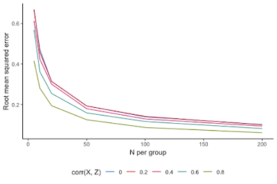
Root mean squared error (RMSE; lower RMSE means greater precision, in other words) is plotted as a function of the sample size (N). Different colors show the increase in precision when you control for covariates with different levels of correlation with the outcome variable. For low levels of correlation with the covariate, you don't get much increase in precision (pink and red lines). Only as the correlation is .6 or above do we see noticeable increases in precision; and it only really makes a big difference with correlations in the range of .8.
Considering these numbers in light of our Dylan study, I would bet that age and writing skill are not correlated with writing skill > .8 (unless we're looking at ages from kindergarten to college!). I would guess that in an adult population this correlation would be much, much lower. So maybe it's not worth controlling for age in our analyses.
And the same is probably true for order, our other covariate. Although perhaps we do think that our order has a strong correlation with our skill measure. For example, maybe our experiment is long and there are big fatigue effects. In that case, we would want to condition.
So these are are options: if the covariate is known to be very strong, we can condition. Otherwise we should probably not worry about it.
What shouldn't we do with our covariates?
Don't condition on lots and lots of covariates because you think they are theoretically important. There are lots of things that people do with covariates that they shouldn't be doing. My personal hunch is that this is because a lot of researchers think that covariates (especially demographic ones like age, gender, socioeconomic status, race, ethnicity, etc.) are important. That's true: these are important variables. But that doesn't mean you need to control for them in every regression. This leads us to the second fallacy.
The second fallacy of covariates is that, because you think covariates are in general meaningful, it is not harmful to control for them in your regression model. In fact, if you control for meaningless covariates in a standard regression model, you will on average reduce your ability to see differences in your treatment effect. Just by chance your noise covariates will "soak up" variation in the response, leaving less to be accounted for by the true treatment effect! Even if you strongly suspect something is a covariate, you should be careful before throwing it into your regression model.
Don't condition on covariates because your groups are unbalanced. People often talk about "unhappy randomization": you randomize adults to the different Dylan groups, for example, but then it turns out the mean age is a bit different between groups. Then you do a t-test or some other statistical test and find out that you actually have a significant age difference. But this makes no sense: because you randomized, you know that the difference in ages occurred by chance, so why are you using a t-test to test if the variation is due to chance? In addition, if your covariate isn't highly correlated with the outcome, this difference won't matter (see above). Finally, if you adjust for this covariate because of such a statistical test, you can actually end up biasing estimates of the ATE across the literature. Here's a really useful blogpost from the Worldbank that has more details on why you shouldn't follow this practice.
Don't condition on covariates post-hoc. The previous example is a special case of a general practice that you shouldn't follow. Don't look at your data and then decide to control for covariates! Conditioning on covariates based on your data is an extremely common route for p-hacking; in fact, it's so common that it shows up in Simmons, Nelson, & Simonsohn's (2011) instant classic False Positive Psychology paper as one of the key ingredients of analytic flexibility. Data-dependent selection of covariates is a quick route to false positive findings that will be less likely to be replicable in independent samples.
Don't condition on a post-treatment variable. As we discussed above, there are some reasons to condition on highly-correlated covariates in general. But there's an exception to this rule. There are some variables that are never OK to condition on – in particular, any variable that is collected after treatment. For example, we might think that another good covariate would be someone's enjoyment of Bob Dylan. So, after the writing measurements are done, we do a Dylan Appreciation Questionnaire (DAQ). The problem is, imagine that having a bad experience writing while listening to Dylan might actually change your DAQ score. So then people in the Dylan condition would have lower DAQ on average. If we control for DAQ in our regression (Y ~ X + DAQ), we then distort our estimate of the effects of Dylan. Because DAQ and X (Dylan condition) are correlated, DAQ will end up soaking up some variance that is actually due to condition. This is bad news. Here's a nice paper that explains this issue in more detail.
Don't condition on a collider. This issue is a little bit off-topic for the current post, since it's primarily an issue in observational designs, but here's a really good blogpost about it.
Conclusions
Covariates and confounds are some of the most basic concepts underlying experimental design and analysis in psychology, yet they are surprisingly complicated to explain. Often the issues seem clear until it comes time to do the data analysis, at which point different assumptions lead to different default analytic strategies. I'm especially concerned that these strategies vary by culture, for example with some psychologists always conditioning on confounders, and others never doing so. (We haven't even talked about mediation and moderation!). Hopefully this post has been useful in using the vocabulary of causal models to explain some of these issues.
---
* The definitive resource on causal graphical models is Pearl (2009). It's not easy going, but it's very important stuff. Even just starting to read it will strengthen your methods/stats muscles.
** Importantly, it's a lot like adding random effects to your model – you model sources of structure in your data so that you can better estimate the particular effects of interest.
*** The advice not to model covariates that aren't very correlated with your outcome is very frequentist, with the idea being that you lose power when you condition on too many things. In contrast, Gelman & Hill (2006) give more Bayesian advice: if you think a variable matters to your outcome, keep it in the model. This advice is consistent with the idea of modeling experimental covariates, even if they don't have a big correlation with the outcome. In the Bayesian framework, including this extra information should (maybe only marginally) improve your precision but you aren't "spending degrees of freedom" in the same way.
Every year, one of the trickiest concepts for me to teach in my experimental methods course is the difference between experimental confounds and covariates. Although this distinction seems simple, it's pretty deeply related to the definition of what an experiment is and why experiments lead to good causal inferences. It's also caught up in a number of methodological problems that come up again and again in my class. This post is my attempt to explain the distinction and how it relates to different problems and cultural practices in psychology.
Throughout this post, I'll use a silly example. My first year of graduate school, I got distracted from my actual research by the hypothesis that listening to music with lyrics decreased my ability to write papers for my classes. I'll call this the "Bob Dylan" hypothesis, since I was listening to a lot of Dylan at the time. Let's represent this by the following causal diagram.

Observational Studies and Experiments
Suppose we did an observational study where we measured each of these variables in a large population. Assume we came up with some way to sample people's writing, get a measure of whether they either were or weren't listening to lyric-heavy music at the time, and assess the writing sample's quality. We might find that Y was correlated with X, but in a surprising direction: listening to Dylan would be related to better writing.
Can we make a causal inference in this case? If so, we could get rich promoting a Dylan-based writing intervention. Unfortunately, we can't – correlation doesn't equal causation here, because there is (at least one) confounding third variable: age (Z). Age is positively related to both Dylan listening and writing skill in our population of interest. Older people tend to be good writers and also tend to be more into folk rockers; I'm not even going to put a question mark on this edge because I'm pretty sure this is true.

To get gold-standard evidence about causality, we need to do an experiment. (We won't discuss statistical techniques for inferring causality, which can be useful but don't give you gold standard evidence anyway; review here).
Experiments are when we intervene on the world and measure the consequences. Here, this means forcing some people to listen to Dylan. In the language of graphical models, if we control the Dylan listening, that means that variable X is causally exogenous. (Exogenous means that it's not caused by anything else in the system). We "snipped" the causal link between age and Dylan listening.

So now we can "wiggle" the Dylan listening variable – change it experimentally – and see if we detect any changes in writing skill. We do this by randomly assigning individuals to listen to Dylan or not and then measuring writing during the assigned listening (or non-listening) period. This is a "between-subjects" design. We can use our randomized experiment to get a measure of the average treatment effect of Dylan, the size of the causal effect of the intervention on the outcome. In this simple experiment, the ATE is estimated by the regression Y ~ X (for ease of exposition, I'm not going to discuss so-called mixed models, which model variation across subjects and/or experimental items). That's the elegant logic of randomized experiments: the difference between condition gives you the average effect.
Confounds
Let's consider an alternate experiment now. Suppose we did the same basic procedure, but now with a "within-subjects" design where participants do both the Dylan treatment and the control, in that order. This experiment is flawed, of course. If you observe a Dylan effect, you can't rule out the idea that participants got tired and wrote worse in the control condition because it always came second.
Order (Dylan first vs. control first; notated X') is an experimental confound: a variable that is created in the course of the experiment that is both causally related to the predictor and potentially also related to the outcome. Here's how the causal model now looks:
We've reconstructed the same kind of confounding relationship we had with age, where we had a variable (X') that was correlated both with our predictor (X) and our outcome (Y)! So...
What should we do with our experimental confounds?
Option 1. Randomize. Increasingly, this is my go-to method for dealing with any confound. Is the correct answer on my survey confounded with response side? Randomize what side the response shows up on! Is order confounded with condition? Randomize the order you present in! Randomization is much easier now that we program many of our experiments using software like Qualtrics or code them from scratch in JavaScript.
The only time you really get in trouble with randomization is when you have a large number of options, a small number of participants, or some combination of the two. In this case, you can end up with unbalanced levels of the randomized factors (for example, ten answers on the right side and two on the left). Averaging across many experiments, this lack of balance will come out in the wash. But in a single experiment, it can really mess up your data – especially if your participants notice and start choosing one side more than the other because it's right more often. For that reason, when balance is critical, you want option 2.
Option 2. Counterbalance. If you think a particular confound might have a significant effect on your measure, balancing it across participants and across trials is a very safe choice. That way, you are guaranteed to have no effect of the confound on your average effect. In a simple counterbalance of order for our Dylan experiment, we manipulate condition order between subjects. Some participants hear Dylan first and others hear Dylan second. Although technically we might call order a second "factor" in the experiment, in practice it's really just a nuisance variable, so we don't talk about it as a factor and we often don't analyze it (but see Option 3 below).
In the causal language we have been using, counterbalancing allows us to snip out the causal dependency between order and Dylan. Now they are unconfounded (uncorrelated) with one another. We've "solved" a confound in our experimental design. Here's the picture:

Counterbalancing doesn't always work, though. It gets trickier when you have too many levels on a variable (too many Dylan songs!) or multiple confounding variables. For example, if you have lots of different nuisance variables – say, condition order, what writing prompt you use for each order, which Dylan song you play – it may not be possible to do a fully-crossed counterbalance so that all combinations of these factors are seen by equal numbers of participants. In these kinds of cases, you may have to rely on partial counterbalancing schemes or latin squares designs, or you may have to fall back on randomization.
Option 3. Do Options 1 and 2 and then model the variation. This option was never part of my training, but it's an interesting third option that I'm increasingly considering.** That is, we are often faced with the choice between A) a noisy between-participants design and B) a lower-noise within-participants design that nevertheless adds noise back in via some obvious order effect that you have to randomize or counterbalance. In a recent talk by Andrew Gelman, he suggested that we try to model these as covariates, to reduce noise. This seems like a pretty interesting suggestion, especially if the correlation between them and the outcome is substantial.***
Covariates
Going back to our example, now we have two variables – age and order – that are no longer confounded with our primary relationship of interest (i.e., Dylan and writing). But they may still be related to our outcome measure. Here's what the picture looks like, repeated from above.
Even if they are not confounding our experimental manipulation, age and experimental condition order may still be correlated with our outcome measure, writing skill. How does this work? Well, the average treatment effect of Dylan on writing is still given by the regression Y ~ X. But we also know that there is some variance in Y that is due to X' and Z.
That's because age and order are covariates: they may – by virtue of their potential causal links with the outcome variable – have some correlation with outcomes, even in a case where the predictor is experimentally manipulated. This should be intuitive for the external (age) covariate, but it's true for both: they may account for variance in Y over and above that controlled by the experimental manipulation of X.
What should we do about our covariates?
Option 1. Nothing! We are totally safe in ignoring all of our covariates, regressing Y on X and treating the estimate as an unbiased estimate of the the effect (the ATE). This is why randomization is awesome. We are guaranteed that, in the limit of many different experiments, even though people with different ages will be in the different Dylan conditions, this source of variation will be averaged out.
The first fallacy of covariates is that, because you have a known covariate, you have to adjust for it. Not true. You can just ignore it and your estimate of the ATE is unbiased. This is the norm in cognitive psychology, for example: variation between individuals is treated as noise and averaged out. Of course, there are weaknesses in this strategy – you will not learn about the relationship of your treatment to those covariates! – but it is sound.
Option 2. If you have a small handful of covariates that you believe are meaningfully related to the outcome, you can plan in advance to adjust for them in your regression. In our Dylan example, this would be a pre-registered plan to add Z as a predictor: Y ~ X + Z. If age (Z) is highly correlated with writing ability (Y), then this will give us a more precise estimate of the ATE, while remaining unbiased.
When should we do this? Well, it turns out that you need a pretty strong correlation to make a big difference. There's some nice code to simulate the effects of covariate adjustment on precision in this useful blogpost on covariate adjustment; I lightly adapted it. Here's the result:

Considering these numbers in light of our Dylan study, I would bet that age and writing skill are not correlated with writing skill > .8 (unless we're looking at ages from kindergarten to college!). I would guess that in an adult population this correlation would be much, much lower. So maybe it's not worth controlling for age in our analyses.
And the same is probably true for order, our other covariate. Although perhaps we do think that our order has a strong correlation with our skill measure. For example, maybe our experiment is long and there are big fatigue effects. In that case, we would want to condition.
So these are are options: if the covariate is known to be very strong, we can condition. Otherwise we should probably not worry about it.
What shouldn't we do with our covariates?
Don't condition on lots and lots of covariates because you think they are theoretically important. There are lots of things that people do with covariates that they shouldn't be doing. My personal hunch is that this is because a lot of researchers think that covariates (especially demographic ones like age, gender, socioeconomic status, race, ethnicity, etc.) are important. That's true: these are important variables. But that doesn't mean you need to control for them in every regression. This leads us to the second fallacy.
The second fallacy of covariates is that, because you think covariates are in general meaningful, it is not harmful to control for them in your regression model. In fact, if you control for meaningless covariates in a standard regression model, you will on average reduce your ability to see differences in your treatment effect. Just by chance your noise covariates will "soak up" variation in the response, leaving less to be accounted for by the true treatment effect! Even if you strongly suspect something is a covariate, you should be careful before throwing it into your regression model.
Don't condition on covariates because your groups are unbalanced. People often talk about "unhappy randomization": you randomize adults to the different Dylan groups, for example, but then it turns out the mean age is a bit different between groups. Then you do a t-test or some other statistical test and find out that you actually have a significant age difference. But this makes no sense: because you randomized, you know that the difference in ages occurred by chance, so why are you using a t-test to test if the variation is due to chance? In addition, if your covariate isn't highly correlated with the outcome, this difference won't matter (see above). Finally, if you adjust for this covariate because of such a statistical test, you can actually end up biasing estimates of the ATE across the literature. Here's a really useful blogpost from the Worldbank that has more details on why you shouldn't follow this practice.
Don't condition on covariates post-hoc. The previous example is a special case of a general practice that you shouldn't follow. Don't look at your data and then decide to control for covariates! Conditioning on covariates based on your data is an extremely common route for p-hacking; in fact, it's so common that it shows up in Simmons, Nelson, & Simonsohn's (2011) instant classic False Positive Psychology paper as one of the key ingredients of analytic flexibility. Data-dependent selection of covariates is a quick route to false positive findings that will be less likely to be replicable in independent samples.
Don't condition on a post-treatment variable. As we discussed above, there are some reasons to condition on highly-correlated covariates in general. But there's an exception to this rule. There are some variables that are never OK to condition on – in particular, any variable that is collected after treatment. For example, we might think that another good covariate would be someone's enjoyment of Bob Dylan. So, after the writing measurements are done, we do a Dylan Appreciation Questionnaire (DAQ). The problem is, imagine that having a bad experience writing while listening to Dylan might actually change your DAQ score. So then people in the Dylan condition would have lower DAQ on average. If we control for DAQ in our regression (Y ~ X + DAQ), we then distort our estimate of the effects of Dylan. Because DAQ and X (Dylan condition) are correlated, DAQ will end up soaking up some variance that is actually due to condition. This is bad news. Here's a nice paper that explains this issue in more detail.
Don't condition on a collider. This issue is a little bit off-topic for the current post, since it's primarily an issue in observational designs, but here's a really good blogpost about it.
Conclusions
Covariates and confounds are some of the most basic concepts underlying experimental design and analysis in psychology, yet they are surprisingly complicated to explain. Often the issues seem clear until it comes time to do the data analysis, at which point different assumptions lead to different default analytic strategies. I'm especially concerned that these strategies vary by culture, for example with some psychologists always conditioning on confounders, and others never doing so. (We haven't even talked about mediation and moderation!). Hopefully this post has been useful in using the vocabulary of causal models to explain some of these issues.
---
* The definitive resource on causal graphical models is Pearl (2009). It's not easy going, but it's very important stuff. Even just starting to read it will strengthen your methods/stats muscles.
** Importantly, it's a lot like adding random effects to your model – you model sources of structure in your data so that you can better estimate the particular effects of interest.
*** The advice not to model covariates that aren't very correlated with your outcome is very frequentist, with the idea being that you lose power when you condition on too many things. In contrast, Gelman & Hill (2006) give more Bayesian advice: if you think a variable matters to your outcome, keep it in the model. This advice is consistent with the idea of modeling experimental covariates, even if they don't have a big correlation with the outcome. In the Bayesian framework, including this extra information should (maybe only marginally) improve your precision but you aren't "spending degrees of freedom" in the same way.
Tuesday, July 23, 2019
An ethical duty for open science?
Let's do a thought experiment. Imagine that you are the editor of a top-flight scientific journal. You are approached by a famous researcher who has developed a novel molecule that is a cure for a common disease, at least in a particular model organism. She would like to publish in your journal. Here's the catch: her proposed paper describes the molecule and asserts its curative properties. You are a specialist in this field, and she will personally show you any evidence that you need to convince you that she is correct – including allowing you to administer this molecule to an animal under your control and allowing you to verify that the molecule is indeed the one that she claims it is. But she will not put any of these details in the paper, which will contain only the factual assertion.
Here's the question: should you publish the paper?
Here's the question: should you publish the paper?
Monday, May 6, 2019
It's the random effects, stupid!
(tl;dr: wonky post on statistical modeling)
I fit linear mixed effects models (LMMs) for most of the experimental data I collect. My data are typically repeated observations nested within subjects, and often have crossed effects of items as well; this means I need to account for this nesting and crossing structure when estimating the effects of various experimental manipulations. For the last ten years or so, I've been fitting these models in lme4 in R, a popular package that allows quick specification of complex models.
One question that comes up frequently regarding these models is what random effect structure to include? I typically follow the advice of Barr et al. (2013), who recommend "maximal" models – models that nest all the fixed effects within a random factor that have repeated observations for that random grouping factor. So for example, if you have observations for both conditions for each subject, fit random condition effects by subject. This approach contrasts, however, with the "parsimonious" approach of Bates et al.,* who argue that such models can be over-parameterized relative to variability in the data. The issue of choosing an approach is further complicated by the fact that, in practice, lme4 can almost never fit a completely maximal model and instead returns convergence warnings. So then you have to make a bunch of (perhaps ad-hoc) decisions about what to prune or how to tweak the optimizer.
Last year, responding to this discussion, I posted a blogpost that became surprisingly popular, arguing for the adoption of Bayesian mixed effects models. My rationale was not mainly that Bayesian models are interpretively superior – which they are, IMO – but just that they allow us to fit the random effect structure that we want without doing all that pruning business. Since then, we've published a few papers (e.g. this one) using Bayesian LMMs (mostly without anyone even noticing or commenting).**
In the mean time, I was working on the ManyBabies project. We finally completed data collection on our first study, a 60+ lab consortium study of babies' preference for infant-directed speech! This is exciting and big news, and I will post more about it shortly. But in the course of data analysis, we had to grapple with this same set of LMM issues. In our pre-registration (which, for what it's worth, was written before I really had tried the Bayesian methods), we said we would try to fit a maximal LMM with the following structure. It doesn't really matter what all the predictors are, but trial_type is the key experimental manipulation:
M1) log_lt ~ trial_type * method +
trial_type * trial_num +
age_mo * trial_num +
trial_type * age_mo * nae +
(trial_type * trial_num | subid) +
(trial_type * age_mo | lab) +
(method * age_mo * nae | item)
Of course, we knew this model would probably not converge. So we preregistered a pruning procedure, which we followed during data analysis, leaving us with:
M2) log_lt ~ trial_type * method +
trial_type * trial_num +
age_mo * trial_num +
trial_type * age_mo * nae +
(trial_type | subid) +
(trial_type | lab) +
(1 | item)
We fit that model and report it in the (under review) paper, and we interpret the p-values as real p-values (well, as real as p-values can be anyway), because we are doing exactly the confirmatory thing we said we'd do. But in the back of my mind, I was wondering if we shouldn't have fit the whole thing with Bayesian inference and gotten the random effect structure that we hoped for.***
So I did that. Using the amazing brms package, all you need to do is replace "lmer" with "brm" (to get a default prior model with default inference).**** Fitting the full LMM on my MacBook Pro takes about 4hrs/chain with completely default parameters, so 16 hrs total – though if you do it in parallel you can fit all four at once. I fit M1 (the maximal model, called "bayes"), M2 (the pruned model, "bayes_pruned"), and for comparison the frequentist (also pruned, called "freq") model. Then I plotted coefficients and CIs against one another for comparison. There are three plots, corresponding to the three pairwise comparisons (brms M1 vs. lme4 M2, brms M1 vs. brms M2, and brms M2 vs. lme4 M2). (So as not to muddy the interpretive waters for ManyBabies, I'm just showing the coefficients without labels here). Here are the results.

As you can see, to a first approximation, there are not huge differences in coefficient magnitudes, which is good. But, inspecting the top row of plots, you can see that the full Bayesian M1 does have two coefficients that are different from both the Bayesian M2 and the frequentist M2. In other words, the fitting method didn't matter with this big dataset – but the random effects structure did! Further, if you dig into the confidence intervals, they are again similar between fitting methods but different between random effects structures. Here's a pairs plot of the correlation between upper CI limits (note that .00 here means a correlation of 1.00!):

Not huge differences, but they track with random effect structure again, not with the fitting method.
In sum, in one important practical case, we see that fitting the maximal model structure (rather than the maximal convergent model structure) seems to make a difference to model fit and interpretation. This evidence to me supports the Bayesian approach that I recommended in my prior post. I don't know that M1 is the best model – I'm trusting the "keep it maximal" recommendation on that point. But to the extent that I should be able to fit all the models I want to try, then using brms (even if it's slower) seems important. So I'm going to keep using this fitting procedure in the immediate future.
----
* This approach seems very promising, but also a bit tricky to implement. I have to admit, I am a bit lazy and it is really helpful when software provides a solution for fitting that I can share with people in my lab as standard practice. A collaborator and I tried someone else's implementation of parsimonious models and it completely failed, and then we gave up. If someone wants to try it on this dataset I'd be happy to share!
* An aside: after I posted, Doug Bates kindly engaged and encouraged me to adopt Julia, rather than R, for model fitting, if it was fitting that I wanted and not Bayesian inference. We did experiment a bit with this, and Mika Braginsky wrote the jglmm package to use Julia for fitting. This experiment resulted in her in-press paper using Julia for model fits, but also with us recognizing that 1) Julia is TONS faster than R for big mixed models, which is a win, but 2) Julia can't fit some of the baroque random effects structures that we occasionally use, and 3) installing Julia and getting everything working is very non-trivial, meaning that it's hard to recommend for folks just getting started.
** Jake Westfall, back in 2016 when we were planning the study, said we should do this, and I basically told him that I thought that developmental psychologists wouldn't agree to it. But I think he was probably right.
*** Code for this post is on github.
I fit linear mixed effects models (LMMs) for most of the experimental data I collect. My data are typically repeated observations nested within subjects, and often have crossed effects of items as well; this means I need to account for this nesting and crossing structure when estimating the effects of various experimental manipulations. For the last ten years or so, I've been fitting these models in lme4 in R, a popular package that allows quick specification of complex models.
One question that comes up frequently regarding these models is what random effect structure to include? I typically follow the advice of Barr et al. (2013), who recommend "maximal" models – models that nest all the fixed effects within a random factor that have repeated observations for that random grouping factor. So for example, if you have observations for both conditions for each subject, fit random condition effects by subject. This approach contrasts, however, with the "parsimonious" approach of Bates et al.,* who argue that such models can be over-parameterized relative to variability in the data. The issue of choosing an approach is further complicated by the fact that, in practice, lme4 can almost never fit a completely maximal model and instead returns convergence warnings. So then you have to make a bunch of (perhaps ad-hoc) decisions about what to prune or how to tweak the optimizer.
Last year, responding to this discussion, I posted a blogpost that became surprisingly popular, arguing for the adoption of Bayesian mixed effects models. My rationale was not mainly that Bayesian models are interpretively superior – which they are, IMO – but just that they allow us to fit the random effect structure that we want without doing all that pruning business. Since then, we've published a few papers (e.g. this one) using Bayesian LMMs (mostly without anyone even noticing or commenting).**
In the mean time, I was working on the ManyBabies project. We finally completed data collection on our first study, a 60+ lab consortium study of babies' preference for infant-directed speech! This is exciting and big news, and I will post more about it shortly. But in the course of data analysis, we had to grapple with this same set of LMM issues. In our pre-registration (which, for what it's worth, was written before I really had tried the Bayesian methods), we said we would try to fit a maximal LMM with the following structure. It doesn't really matter what all the predictors are, but trial_type is the key experimental manipulation:
M1) log_lt ~ trial_type * method +
trial_type * trial_num +
age_mo * trial_num +
trial_type * age_mo * nae +
(trial_type * trial_num | subid) +
(trial_type * age_mo | lab) +
(method * age_mo * nae | item)
Of course, we knew this model would probably not converge. So we preregistered a pruning procedure, which we followed during data analysis, leaving us with:
M2) log_lt ~ trial_type * method +
trial_type * trial_num +
age_mo * trial_num +
trial_type * age_mo * nae +
(trial_type | subid) +
(trial_type | lab) +
(1 | item)
We fit that model and report it in the (under review) paper, and we interpret the p-values as real p-values (well, as real as p-values can be anyway), because we are doing exactly the confirmatory thing we said we'd do. But in the back of my mind, I was wondering if we shouldn't have fit the whole thing with Bayesian inference and gotten the random effect structure that we hoped for.***
So I did that. Using the amazing brms package, all you need to do is replace "lmer" with "brm" (to get a default prior model with default inference).**** Fitting the full LMM on my MacBook Pro takes about 4hrs/chain with completely default parameters, so 16 hrs total – though if you do it in parallel you can fit all four at once. I fit M1 (the maximal model, called "bayes"), M2 (the pruned model, "bayes_pruned"), and for comparison the frequentist (also pruned, called "freq") model. Then I plotted coefficients and CIs against one another for comparison. There are three plots, corresponding to the three pairwise comparisons (brms M1 vs. lme4 M2, brms M1 vs. brms M2, and brms M2 vs. lme4 M2). (So as not to muddy the interpretive waters for ManyBabies, I'm just showing the coefficients without labels here). Here are the results.


Not huge differences, but they track with random effect structure again, not with the fitting method.
In sum, in one important practical case, we see that fitting the maximal model structure (rather than the maximal convergent model structure) seems to make a difference to model fit and interpretation. This evidence to me supports the Bayesian approach that I recommended in my prior post. I don't know that M1 is the best model – I'm trusting the "keep it maximal" recommendation on that point. But to the extent that I should be able to fit all the models I want to try, then using brms (even if it's slower) seems important. So I'm going to keep using this fitting procedure in the immediate future.
----
* This approach seems very promising, but also a bit tricky to implement. I have to admit, I am a bit lazy and it is really helpful when software provides a solution for fitting that I can share with people in my lab as standard practice. A collaborator and I tried someone else's implementation of parsimonious models and it completely failed, and then we gave up. If someone wants to try it on this dataset I'd be happy to share!
* An aside: after I posted, Doug Bates kindly engaged and encouraged me to adopt Julia, rather than R, for model fitting, if it was fitting that I wanted and not Bayesian inference. We did experiment a bit with this, and Mika Braginsky wrote the jglmm package to use Julia for fitting. This experiment resulted in her in-press paper using Julia for model fits, but also with us recognizing that 1) Julia is TONS faster than R for big mixed models, which is a win, but 2) Julia can't fit some of the baroque random effects structures that we occasionally use, and 3) installing Julia and getting everything working is very non-trivial, meaning that it's hard to recommend for folks just getting started.
** Jake Westfall, back in 2016 when we were planning the study, said we should do this, and I basically told him that I thought that developmental psychologists wouldn't agree to it. But I think he was probably right.
*** Code for this post is on github.
Monday, April 8, 2019
A (mostly) positive framing of open science reforms
I don't often get the chance to talk directly and openly to people who are skeptical of the methodological reforms that are being suggested in psychology. But recently I've been trying to persuade someone I really respect that these reforms are warranted. It's a challenge, but one of the things I've been trying to do is give a positive, personal framing to the issues. Here's a stab at that.
My hope is that a new graduate student in the fields I work on – language learning, social development, psycholinguistics, cognitive science more broadly – can pick up a journal and choose a seemingly strong study, implement it in my lab, and move forward with it as the basis for a new study. But unfortunately my experience is that this has not been the case much of the time, even in cases where it should be. I would like to change that, starting with my own work.
Here's one example of this kind of failure: As a first-year assistant professor, a grad student and I tried to replicate one of my grad school advisors' well-known studies. We failed repeatedly – despite the fact that we ended up thinking the finding was real (eventually published as Lewis & Frank, 2016, JEP:G). The issue was likely that the original finding was an overestimate of the effect, because the original sample was very small. But converging on the truth was very difficult and required multiple iterations.
Thursday, February 21, 2019
Nothing in childhood makes sense except in the light of continuous developmental change
I'm awestruck by the processes of development that operate over children's first five years. My daughter M is five and my newborn son J is just a bit more than a month old. J can't yet consistently hold his head up, and he makes mistakes even in bottle feeding – sometimes he continues to suck but forgets to swallow so that milk pours out of his mouth until his clothes are soaked. I remember this kind of thing happening with M as a baby ... and yet voila, five years later, you have someone who is writing text messages to grandma and illustrating new stories about Spiderman. How you could possibly get from A to B (or in my case, from J to M)? The immensity of this transition is perhaps the single most important challenge for theories of child development.
As a field, we have bounced back and forth between continuity and discontinuity theories to explain these changes. Continuity theories posit that infants' starting state is related to our end state, and that changes are gradual, not saltatory; discontinuity theories posit stage-like transitions. Behaviorist learning theory was fundamentally a continuity hypothesis – the same learning mechanisms (plus experience) underly all of behavior, and change is gradual. In contrast, Piagetian stage theory was fundamentally about explaining behavioral discontinuities. As the pendulum swung, we get core knowledge theory, a continuity theory: innate foundations are "revised but not overthrown" (paraphrasing Spelke et al. 1992). Gopnik and Wellman's "Theory theory" is a discontinuity theory: intuitive theories of domains like biology or causality are discovered like scientific theories. And so on.
For what it's worth, my take on the "modern synthesis" in developmental psychology is that development is domain-specific. Domain of development – perception, language, social cognition, etc. – progress on their own timelines determined by experience, maturation, and other constraining factors. And my best guess is that some domains develop continuously (especially motor and perceptual domains) while others, typically more "conceptual" ones, show more saltatory progress associated with stage changes. But – even though it would be really cool to be able to show this – I don't think we have the data to do so.
The problem is that we are not thinking about – or measuring – development appropriately. As a result, what we end up with is a theoretical mush. We talk as though everything is discrete, but that's mostly a function of our measurement methods. Instead, everything is at rock bottom continuous, and the question is how steep the changes are.
We talk as though everything is discontinuous all the time. The way we know how to describe development verbally is through what I call "milestone language." We discuss developmental transitions by (often helpful) age anchors, like "children say their first word around their first birthday," or "preschoolers pass the Sally-Ann task at around 3.5 years." When summarizing a study, we* assert that "by 7 months, babies can segment words from fluent speech," even if we know that this statement describes the fact that the mean performance of a group is significantly different than zero in a particular paradigm instantiating this ability, and even if we know that babies might show this behavior a month earlier if you tested enough of them! But it's a lot harder to say "early word production emerges gradually from 10 - 14 months (in most children)."
Beyond practicalities, one reason we use milestone language is because our measurement methods are only set up to measure discontinuities. First, our methods have poor reliability: we typically don't learn very much about any one child, so we can't say conclusively whether they truly show some behavior or not. In addition, most developmental studies are severely underpowered, just like most studies in neuroscience and psychology in general. So the precision of our estimates of a behavior for groups of children are noisy. To get around this problem, we use null hypothesis significance tests – and when the result is p < .05, we declare that development has happened. But of course we will see discrete changes in development if we use a discrete statistical cutoff!
And finally, we tend to stratify our samples into discrete age bins (which is a good way to get coverage), e.g. recruiting 3-month-olds, 5-month-olds, and 7-month-olds for a study. But then, we use these discrete samples as three separate analytic groups, ignoring the continuous developmental variation between them! This practice reduces statistical power substantially, much like taking median splits on continuous variables (taking a median split on average is like throwing away a third of your sample!). In sum, even in domains where development is continuous, our methods guarantee that we get binary outcomes. We don't try to estimate continuous functions, even when our data afford them.
The truth is, when you scratch the surface in development, everything changes continuously. Even the stuff that's not supposed to change still changes. I saw this in one of my very first studies, when I was a lab manager for Scott Johnson and we accidentally found ourselves measuring 3-9 month-olds' face preferences. Though I had learned from the literature that infants had an innate face bias, I was surprised to find that magnitude of face looking was changing dramatically across the range I was measuring. (Later we found that this change was related to the development of other visual orientating skills). Of course "it's not surprising" that some complex behavior goes up with development, says reviewer 3. But it is important, and the ways we talk about and analyze our data don't reflect the importance of quantifying continuous developmental change.
One reason that it's not surprising to see developmental change is that everything that children do is at its heart a skill. Sucking and swallowing is a skill. Walking is a skill. Recognizing objects is a skill. Recognizing words is a skill too - so too is the rest of language, at least according to some folks. Thinking about other people's thoughts is a skill. So that means that everything gets better with practice. It will – to a first approximation – follow a classic logistic curve like this:

Most skills get better with practice, and the ones described above are no exception. But developmental progress also happens in the absence of practice of specific skills due to physiological maturation – older children's brains are faster and more accurate at processing information, even for skills that haven't been practiced. So samples from this behavior should look like these red lines:

But here's the problem. If you have a complex behavior, it's built of simple behaviors, which are themselves skills. To get the probability of success on one of those complex skills, you can – as a first approximation – multiply the independent probabilities of success in each of the components. That process yields logistic curves that look like these (color indicating the number of components):

And samples from a process with many components look even more discrete, because the logistic is steeper!

Given this kind of perspective, we should expect complex behaviors to emerge relatively suddenly, even if they are simply the product of a handful of continuously changing processes.
This means, from a theoretical standpoint, we need stronger baselines. Our typical baseline at the moment is the null hypothesis of no difference; but that's a terrible baseline! Instead, we need to be comparing to a null hypothesis of "developmental business as usual." To show discontinuity, we need to take into account the continuous changes that a particular behavior will inevitably be undergoing. And then, we need to argue that the rate of developmental change that a particular process is undergoing is faster than we should expect based on simple learning of that skill. Of course to make these kinds of inferences requires far more data about individuals than we usually gather.
---
* I definitely do this too!
As a field, we have bounced back and forth between continuity and discontinuity theories to explain these changes. Continuity theories posit that infants' starting state is related to our end state, and that changes are gradual, not saltatory; discontinuity theories posit stage-like transitions. Behaviorist learning theory was fundamentally a continuity hypothesis – the same learning mechanisms (plus experience) underly all of behavior, and change is gradual. In contrast, Piagetian stage theory was fundamentally about explaining behavioral discontinuities. As the pendulum swung, we get core knowledge theory, a continuity theory: innate foundations are "revised but not overthrown" (paraphrasing Spelke et al. 1992). Gopnik and Wellman's "Theory theory" is a discontinuity theory: intuitive theories of domains like biology or causality are discovered like scientific theories. And so on.
For what it's worth, my take on the "modern synthesis" in developmental psychology is that development is domain-specific. Domain of development – perception, language, social cognition, etc. – progress on their own timelines determined by experience, maturation, and other constraining factors. And my best guess is that some domains develop continuously (especially motor and perceptual domains) while others, typically more "conceptual" ones, show more saltatory progress associated with stage changes. But – even though it would be really cool to be able to show this – I don't think we have the data to do so.
The problem is that we are not thinking about – or measuring – development appropriately. As a result, what we end up with is a theoretical mush. We talk as though everything is discrete, but that's mostly a function of our measurement methods. Instead, everything is at rock bottom continuous, and the question is how steep the changes are.
We talk as though everything is discontinuous all the time. The way we know how to describe development verbally is through what I call "milestone language." We discuss developmental transitions by (often helpful) age anchors, like "children say their first word around their first birthday," or "preschoolers pass the Sally-Ann task at around 3.5 years." When summarizing a study, we* assert that "by 7 months, babies can segment words from fluent speech," even if we know that this statement describes the fact that the mean performance of a group is significantly different than zero in a particular paradigm instantiating this ability, and even if we know that babies might show this behavior a month earlier if you tested enough of them! But it's a lot harder to say "early word production emerges gradually from 10 - 14 months (in most children)."
Beyond practicalities, one reason we use milestone language is because our measurement methods are only set up to measure discontinuities. First, our methods have poor reliability: we typically don't learn very much about any one child, so we can't say conclusively whether they truly show some behavior or not. In addition, most developmental studies are severely underpowered, just like most studies in neuroscience and psychology in general. So the precision of our estimates of a behavior for groups of children are noisy. To get around this problem, we use null hypothesis significance tests – and when the result is p < .05, we declare that development has happened. But of course we will see discrete changes in development if we use a discrete statistical cutoff!
And finally, we tend to stratify our samples into discrete age bins (which is a good way to get coverage), e.g. recruiting 3-month-olds, 5-month-olds, and 7-month-olds for a study. But then, we use these discrete samples as three separate analytic groups, ignoring the continuous developmental variation between them! This practice reduces statistical power substantially, much like taking median splits on continuous variables (taking a median split on average is like throwing away a third of your sample!). In sum, even in domains where development is continuous, our methods guarantee that we get binary outcomes. We don't try to estimate continuous functions, even when our data afford them.
One reason that it's not surprising to see developmental change is that everything that children do is at its heart a skill. Sucking and swallowing is a skill. Walking is a skill. Recognizing objects is a skill. Recognizing words is a skill too - so too is the rest of language, at least according to some folks. Thinking about other people's thoughts is a skill. So that means that everything gets better with practice. It will – to a first approximation – follow a classic logistic curve like this:


But here's the problem. If you have a complex behavior, it's built of simple behaviors, which are themselves skills. To get the probability of success on one of those complex skills, you can – as a first approximation – multiply the independent probabilities of success in each of the components. That process yields logistic curves that look like these (color indicating the number of components):

And samples from a process with many components look even more discrete, because the logistic is steeper!

Given this kind of perspective, we should expect complex behaviors to emerge relatively suddenly, even if they are simply the product of a handful of continuously changing processes.
This means, from a theoretical standpoint, we need stronger baselines. Our typical baseline at the moment is the null hypothesis of no difference; but that's a terrible baseline! Instead, we need to be comparing to a null hypothesis of "developmental business as usual." To show discontinuity, we need to take into account the continuous changes that a particular behavior will inevitably be undergoing. And then, we need to argue that the rate of developmental change that a particular process is undergoing is faster than we should expect based on simple learning of that skill. Of course to make these kinds of inferences requires far more data about individuals than we usually gather.
In a conference paper that I'm still quite proud of, we tried to create this sort of baseline for early word learning. Arguably, early word learning is a domain where there likely aren't huge, discontinuous changes – instead kids gradually get faster and more accurate in learning new words until they are learning several new words per day. We used meta-analysis to estimate developmental increases in two component processes of novel word mapping: auditory word recognition and social cue following. Both of these got faster and more accurate over the first couple of years. When we put these increases together, we found they together created really substantial changes in how much input would be needed for a new word mapping. (Of course what we haven't done in the three years since we wrote that paper is actually measure the parameters on the process of word mapping developmentally – maybe that's for a subsequent ManyBabies study...). Overall, this baseline suggests that even in the absence of discontinuity, continuous changes in many small processes can produce dramatic developmental differences.
In sum: sometimes developmental psychologists don't take the process of developmental change seriously enough. To do better, we need to start analyzing change continuously; measuring with sufficient precision to estimate rates of change; and creating better continuous baselines before we make claims about discrete change or emergence.
In sum: sometimes developmental psychologists don't take the process of developmental change seriously enough. To do better, we need to start analyzing change continuously; measuring with sufficient precision to estimate rates of change; and creating better continuous baselines before we make claims about discrete change or emergence.
---
* I definitely do this too!
Subscribe to:
Posts (Atom)